Are there times when, when opening Excel, you get lost in numerous negative numbers, and the only possible way you see to change it is by manually turning each of them into a positive? You would certainly like to know the easiest way to change all this. Well, you get your paws on some magical techniques about how to transform negative figures into positive ones in Excel with just one click or two.
In this regard, today’s article reveals the top four foolproof methods to choose from any complex formulas. All of these techniques will guide you through a sequence of steps. You will also receive pictures of the steps related to it all in one. Is there any chance left behind of not becoming an Excel expert? The answer is a striking no!
Then, let’s go back to how to turn negative things into positive things using Excel. We know you won’t want to miss a single word until the conclusion.
How to Make a Negative Number Positive in Excel Via Paste Special?
Paste Special is, in fact, one of the easiest tricks for turning negative numbers into positive ones within a few clicks. This technique’s magic is to write -1 in a different cell and perform several other operations on the data. This conversion can be done in the same column or a different column.
Do you wish to learn how a positive number can be obtained from a negative one in Excel? Here are the comprehensive guidelines to help you work on Excel like a professional.
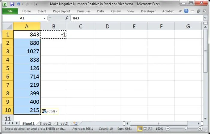
Imagine we have the following data set from which we will attempt to convert negatives into positives:
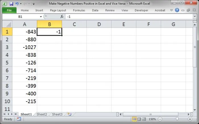
Step 1: Start by placing the value – 1 in a cell close to the place where the negative numbers are placed.
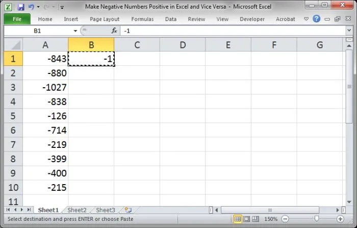
Step 2: Now, we have to right-click on the cell containing -1 and select the command ‘copy.’ You could also call Ctrl+C or possibly a couple of Ctrl+C.
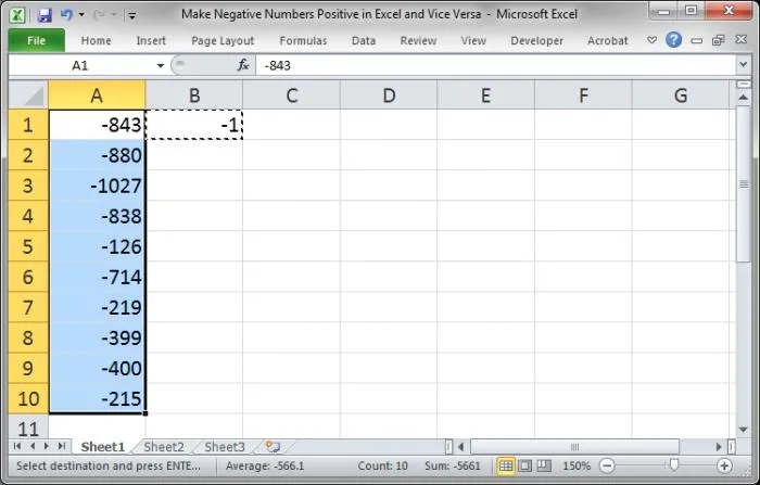
Step 3: To make the selected negative numbers positive, set the cursor on the selected cells containing the negative numbers.
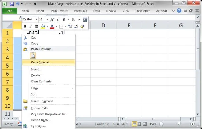
Step 4: Right-click the mouse, then go to Paste Special on the rapidly appearing option, choosing the target choice. Otherwise, you can go for the quick way and use the shortcut Ctrl+Alt+V. Doing that will take you to the Paste Special dialogue box.
Step 5: Carefully choose the option “All”.
Step 6: To add positivity to each number, click the ‘Multiply‘ button, and to finalise the deal, click OK.’
Step 7: All the negative numbers have disappeared into the air, leaving you with a column of positive ones. Woohoo!
Step 8: The end would be to remove the -1, and then it is set.
How to Make Negative Numbers Positive in Excel Via Simple Formula
You know the basic arithmetic we have always been taught in class, where we learn that minus multiplied by minus equals a plus? That is how a simple formula is used in Excel. Based on this method, negativity, if multiplied by negativity, negates both, giving positivity.
Are you still in a position where we need to assist you with how to convert negative numbers to positive ones in Excel? Here you go!
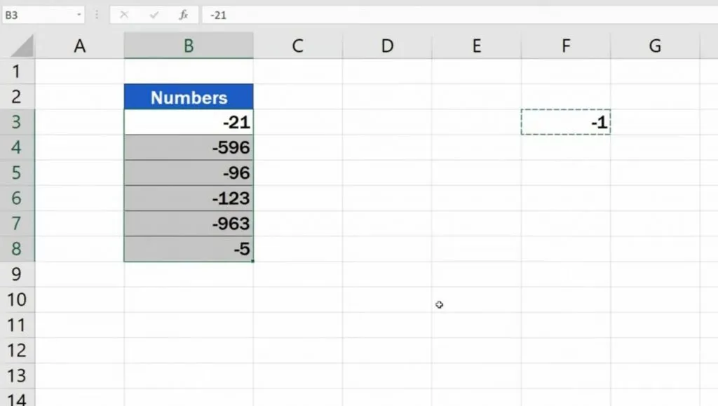
For instance, assume you have the following data set in column B and wish to have their positives appear in column D.
Step 1: Inscribe -1 in the cell of a desired row in column F.

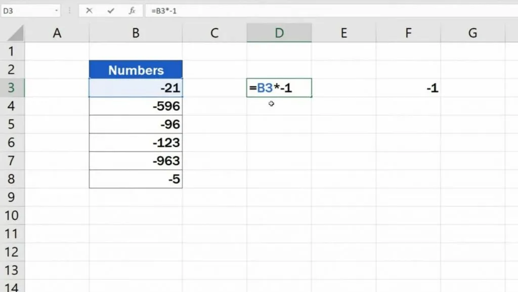
Step 2: Select the cell for which you want to use the simple formula, type an equal (=) sign, and select the number with a negative sign that you want to make positive. As soon as you write it into the cell, you will get B3 written in the cell. Multiply it by -1. In this manner, negative values will be converted to positive numbers.
Step 3: To make all the values positive, select a cell with a positive number and copy it. Then, right-click and drag it down to the cell that needs to be made positive. Ta-dah! You have triumphed in the magical way of turning negative values into positive ones.
How to Convert Negative to Positive in Excel Via Flash Fill?
Flash Fill method is the final blow to repeated use of your eraser, and the most efficient way to convert from negative to positive in an Excel worksheet. This technique involves the identification of a pattern, and then the data is completed on its own. You have to include one or two from each as an example. And the rest of all is to be done with this method automatically, which simply means that the investment of effort in this case is minimal. Therefore, it can turn negatives into positives as if it were a piece of cake.
Would you be interested in applying this method? Below is the outline of each step, which can guide you through the process ahead.
So, let’s assume this is the dataset that has been given to us with the aim of transforming the negatives into positives.
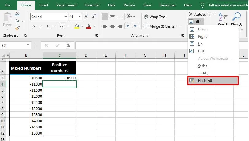
Step 1: The next step is to add up the first value without a minus to the first cell of the column next to your negative numbers.
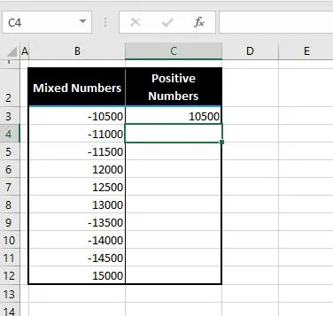
Step 2: Choose any of the targeted cells and go towards the Home Tab: Move the arrow towards the Fill button placed in the Editing group and hit the button. Searching for a Flash Fill option? Click it and watch the wonders work!
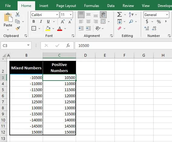
Step 3: After locating the compatible pattern, Flash Fill will apply the transformations and convert all the negative values into positive values. Check it out!
How to Turn Negative to Positive in Excel Via ABS?
ABS is a very important technique in Excel that transforms negatives into positives within a blink of an eye. This absolute method eliminates the sign from a number and gives the absolute value of the same in Microsoft Excel. Do you record all positive data, or do mathematical calculations involve finance? Whether it is so, the ABS method is sure to transform your approach to data.
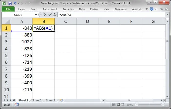
So, do you want to know how to swim in Excel by force and transform negative values into positives with the help of ABS? Here is the entire data set, with all the negative values in the only column that needs to be transformed into positives.
Step 1: To begin with, inside an empty cell of column B, insert the secret formula =ABS(Cell reference) and then press enter. You’ll get the positive value in the B1 cell.
Step 2: Wait, there’s more. You can do this to the whole column you want to make positive. To copy the formula down drag the cell from the bottom right corner. If you do this, then the formula enters the formula down into the row.
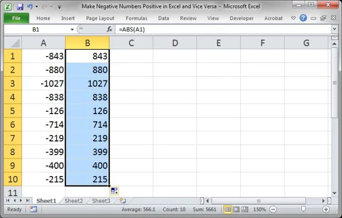
Now, column B has all the absolute values of all the numbers in column A of our Excel spreadsheet.

