Microsoft Excel is one of the best freely available spreadsheet tools; moreover, since the tool permits having several sheets within a single file, things can only improve. However, there are times when you want to compare sheets for different or even the same values in the data, and if you do not know the right process, depending on the size of the data involved, this can take time. Find out how to compare two Excel sheets effectively to reduce the amount of time taken.
Now, let us discuss the top 5 easy ways to compare 2 different Excel sheets and look for differences and/or matching data. The beauty of it is that all the methods listed above save time.
How do you compare two Excel sheets for differences and duplicates with “Arrange all”?
The first method we will elaborate on here is the Arrange All function of Microsoft Excel. It is also much less complicated than other methods that are used, and the preparation process is quicker and requires fewer actions. So, here are all the steps to follow for using the Arrange All method:
- Click on the file and Excel sheets to compare, and click on the tab view. Now click the ‘side by side‘ button. A word of caution here is that this button is only active when several Microsoft Excel spreadsheets are running.
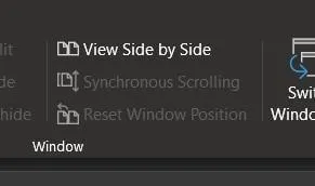
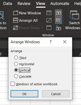
- Any Excel spreadsheet created will default to being horizontally formatted. Therefore, you need to click the Arrange All button and choose Vertical.
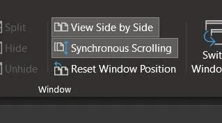
- The last thing required to facilitate comparisons is synchronizing scrolling in the view section. Enabling it means that these two sheets will scroll in tandem.

It can be used if you have two sheets in two different Excel documents or one document. Furthermore, apply this method when working with a small dataset since you can easily make mistakes. Although this method will be time-consuming, it will save you much more time than the whole process alone.
How do you compare two Excel sheets for duplicates or differences with a “New window”?
The New Window method is another comparative technique for data in Excel sheets. It is especially useful when you have one workbook but different sheets within it. It also allows for comparing different Excel workbooks, selecting them in the desired order so the application can compare them and show the differences or identities between the files.
This is possible thanks to the launched feature named New Window from Excel, and the way it is done is not complicated, unlike the previous one. Let’s take the example of one workbook with 2 spreadsheets in it that you will compare with the following steps:
- Before working on the Microsoft Excel workbook and spreadsheets, you must change the view and select the new window option. This will open another window for the same Excel worksheet.

- If one or all of these windows are horizontally aligned but you wish to match or contrast data in columns, click the Arrange All button to align vertically.

- However, enabling the synchronous scrolling option under the view tab is useful if your spreadsheets have long data columns. This links both spreadsheets so that the rows function as if they synchronize; if you scroll down the rows of one, the same thing happens to the second one.
This method is better for small data sets since you must compare the data independently. While comparing the data, you may encounter the human error factor. Furthermore, it performs very well with one workbook and two sheets.
How do you compare two Excel sheets and highlight differences?
One thing that many of the previous two methods suggest is that you have to compare data by hand. That is only possible if you have only a few rows as each column on your chart or table. If your columns are longer, it will give several errors in that method, and that’s why it’s wise to look for a smart way. However, if you want to compare the differences, make sure that you use smart tools from Excel.
The best part is that the differences were made very clear. However, having the spreadsheets in one workbook is important, as you cannot open two workbooks side by side to compare with this method. If you have spreadsheets in several workbooks, you can paste them into one.
To elaborate further, let’s consider two datasets; one has newly calculated student scores, and the other has old scores. It uses the Conditional Formatting feature, and here are the steps to implement this method:
- Go to the “New” sheet, right-click the cursor pointing at the data area, choose the home tab at the top, and click conditional formatting and new rules.

- In the rules section, you need to tick the last option where you choose cells and enter the formula in the formula field as =B2<>Old!B2 Replace the parameters based on the name of your column and the spreadsheet.
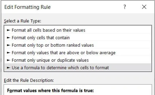
To format the cell after entering the formula, hit the format button. Finally, choose a color from the Fill tab in the opened popup window and press OK. Now you see that the different values will be underlined immediately.
How do you compare two Excel sheets and highlight differences online?
If that’s difficult to work with, switch to an even smarter solution. The proposed solution includes keeping records in an online archive called Google Sheets. This tool permits the import of files with the extension XLSX. Because both use the spreadsheet interface, it also shows your Excel workbook.
However, it operates with the same conditional formatting approach, although it is different somehow. Here, the comparison is performed in one phase, and the highlight is in the other phase. Say that you have uploaded your Excel workbook with 2 spreadsheets to Google Sheets and opened it; now you can follow the steps below to find differences:
- You just select the blank cell you wish to format and type an equal sign. After this, you want to click on the cell from the first spreadsheet you want to compare with the other one. Once more, type the equal sign, navigate to the second spreadsheet in this document, and select the first-row data cell. When you press the hit enter, you will get an option either true/false.
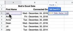
- After that fill formula in that column by activating the right corner of the cell of the first row and dragging it down. For instance, you will find true/false brands indicated in each cell. When the contents of the selected cells have equal values, a true is depicted, while if the contents differ, a false is depicted.
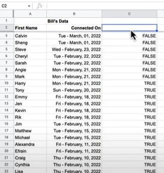
- Choose the column being compared with the other data in the table. Right from the homepage menu bar, click on format followed by conditional formatting. Going to the labeled format cells section, choose the conditional formula. In the formula bar, the input will be “=C3=F“. The formula for the computation of N is that C3 is a True/False column, and if you use some other column for True/False, then replace C3 with that and 3 with the first entry of that column. Finally, you are required to choose a color and press the Done button.
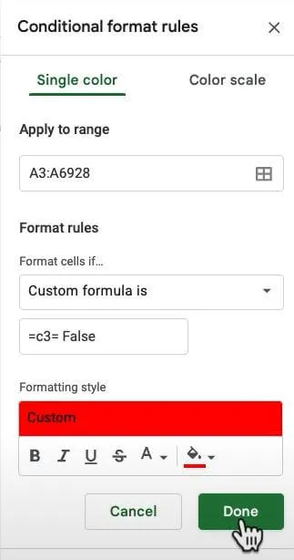
You will find that all these various values are highlighted immediately from here onwards.
How do you compare two sheets in Excel for matches and highlight them?
Before we turn to how that information is extracted and called out, we have investigated how that differential data may be discovered. Let’s explain how to find the matching data or duplicates between the sheets and how to highlight them. The process is relatively easy since the tactic also employs conditional formatting. Here the only thing that will change is the formula. The steps and processes will also remain the same.
However, for this method to be effective, both sheets should be in one Excel workbook since the conditional formatting option is unavailable when the data is split into two workbooks. One solution is to copy it into a different sheet within your workbook. Let’s use the same example of new and old sheets with columns heading to student scores. So, find matching data and highlight them using the following steps:
- Grab the mouse and click over the “New” sheet to select the data in the sheet. On the home tab, click the conditional formatting option, then click on the new rules option.
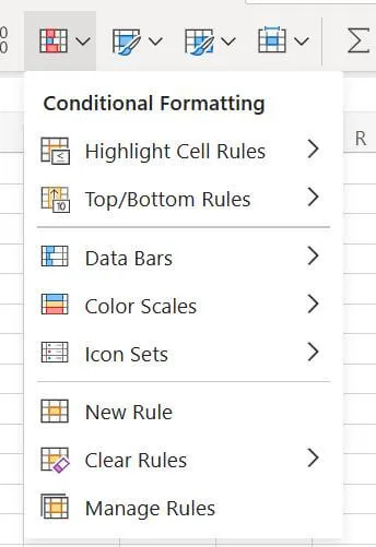
On this screen, select the option that uses the formula for cell formatting. After typing it in a formula bar, type the formula as “=B2=Old!B2.” Please substitute this formula with your column and the name of your spreadsheet.

Finally, at the end of the last step, you will see that those values are highlighted to show that they match.

