While working with large data sets, duplicate information is frustrating and time-consuming in Excel. Whether you seek information from different websites or ask your colleagues for help, there are always some redundancies in the work, and it is hard to find all the redundancies in Excel.
This comprehensive and informative article will outline how to quickly look for and eliminate duplicates in a large Excel worksheet. This will allow you to save time and ensure that your data is accurate.
How do you find duplicates in Excel without deleting them but by highlighting them?
It is relatively easy to establish, expound, and elucidate duplicate cells in Excel without eradicating the cells. If you want to find the duplicates and highlight them in Excel then there is a plenty of in-built rule with which you can do this effortlessly well, one of them is described below.
To effectively apply this rule and resolve how to find duplicates in Excel problem, follow these steps:
Step 1: Open the Windows file search and type Excel. You must open the workbook first to edit the workbook or just the file. To perform this calculation on a range of data, simply select the data or select an entire column in which you want to look for duplicates.
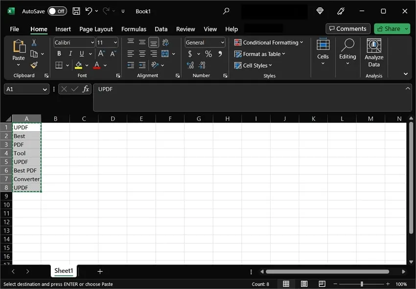
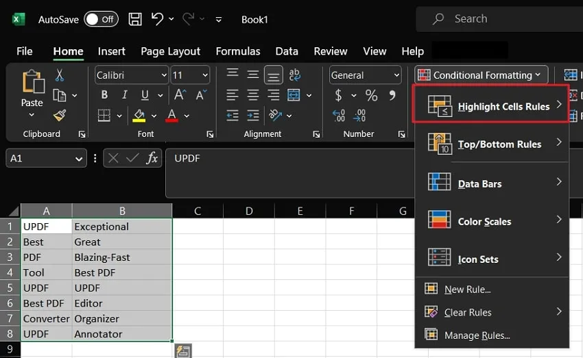
Step 2: Then click on the “Home” tab at the top of the interface and find “Conditional Formatting” in the menu. Double-tap it, go to the “Highlight Cells Rules” menu within the dropdown, and choose “Duplicate Values.” You can now select any value in the “Values With” drop-down list and click the “OK” button to apply formatting.
How Do I Find Duplicates in Excel But Keep One?
Of all the Excel parameters, the Remove Duplicates feature best identifies duplicates while retaining one value. Carry out the steps below to utilize this feature:
Step 1: Choose the required data, which may be a column or any specific range present in your Excel workbook. Go to the menu bar and find the “Data” option on the tab opened, then tools in data with a group of “Data Tools.” Click the “Remove Duplicates” icon to launch the relevant dialog in this group.
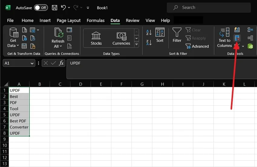
Step 2: Now, you can confirm the selected column or input any other values and click the “OK” button. This will bring a message box with the values that were found, removed, and those that remained. Choose “OK,” and the changes have been made.
How do you use Formulas to find duplicates in Excel?
Perform a search formula in Excel to avoid cases of duplication of entries and manage your analytical work in Excel to identify duplications easily. You can easily look for duplicate values if you have implemented the required function. However, do not forget that the above formula compares duplicate or original with the said value. Try the below-outlined steps:
Step 1: If you have an Excel file open to the position where the reader needs it, insert into the formula bar the following: =IF(COUNTIF($A$2:$A$8, $AA)>1, “Duplicate,” “Unique“). Don’t forget to make the correct cell active where you want the copied formula before copy-pasting.
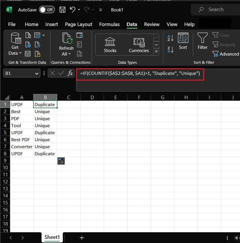
Step 2: Now edit this function to choose the needed data cells where the formula should be used. However, if this is done, press the ‘Enter‘ button on the keyboard to view the results. By the way, the $A1 will be the input from the first cell of your data field.
How do you find duplicates in Excel between two columns?
It is very easy to search for duplicates in Excel for two columns. You can follow the below-mentioned steps to identify any duplicate entries in your spreadsheet across multiple columns:
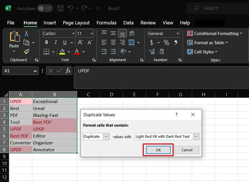
Step 1: On your Excel sheet, you need to choose several columns of data to perform the necessary operations. Then go to ‘Home,’ click the drop-down list next to ‘Conditional formatting,’ and select the ‘Highlight Cells Rules‘ sub-option.
Step 2: Next, from the outlined “Highlight Cells Rules,” choose “Duplicate Values,” which will open the “Duplicate Values” dialogue box. Select the shades of the color different for the results, then click on the “OK” button. This will make it easier for everyone to see all the same values repeated in different columns.
How do you find duplicates in Excel between two sheets?
Would you like to know what kind of copy-paste mistakes are possible in two different Excel sheets? But there are many ways of including this technique in your Excel, and we will explain the simplest method to avoid confusing you.
Follow the straightforward instructions below to compare and find duplicates in two Excel sheets:
Step 1: Open the Excel file, click the sheet from where you want to delete duplicates, copy the data from sheet 1, and paste it into B1 of sheet 2. Then, click “Conditional Formatting” and choose the “New Rules” option from the list that appears.
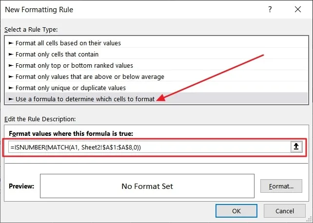
Step 2: From the “New Formatting Rule” window, identify and go with the “Use a formula to determine which cells to format” rule type. Next, copy and paste this formula “=ISNUMBER(MATCH(A1, Sheet2!$A$1:The following formula should be inserted into the blank space mentioned above by replacing 8.0 with your data: “$A $8,0“.
Step 3: After this, press the ‘Format‘ button, and under ‘Fill,’ choose the color you want to use to color the duplicated data cells. Then, press the “OK” buttons in the opened windows to search for similar values in the two Excel sheets.


